2024 Forecast Methodology
The Decision Desk HQ 2024 forecasting model provides the probability of each candidate winning each state in the presidential election, the mean expected electoral vote total for each candidate, and the overall probability of each candidate winning the Electoral College and thus the presidency. Additionally, the model is designed to produce accurate estimates of the probability of Republican and Democratic victories in individual House and Senate elections, as well as the aggregate number of seats expected to be won by each party in the Senate and House. The model is built upon the framework of previous models in 2020 and 2022, with some methodological improvements.
Summary
Our dataset comprises over 200 base features including economic indicators, measures of the political environment (both national and local), candidate traits, and campaign finance reports. We also include engineered variables designed to draw context-specific information into the model. We refresh this dataset on a rolling basis. Not all features are used in every estimator; many are most effective when paired with certain other features and estimators. We also create adjusted variables from various data points, such as an adjusted PVI metric that combines the PVI with our generic ballot average, serving as one of our model's many predictors.
We use Bayesian ridge regression, random forest, gradient boosting, and ElasticNet regression which when ensembled prove to be more accurate (Montgomery et al. 2011). Finally, we complete the ensemble by incorporating a weighted and bias-corrected polling average when available to produce our final prediction. We then run correlated simulations on our predictions to derive the range of possible outcomes.
Our quantitative estimates for each race are converted into qualitative ratings, as described in Figure 1 below. This is done in an entirely automated fashion—we set the bounds on the ratings and go wherever the model takes us.
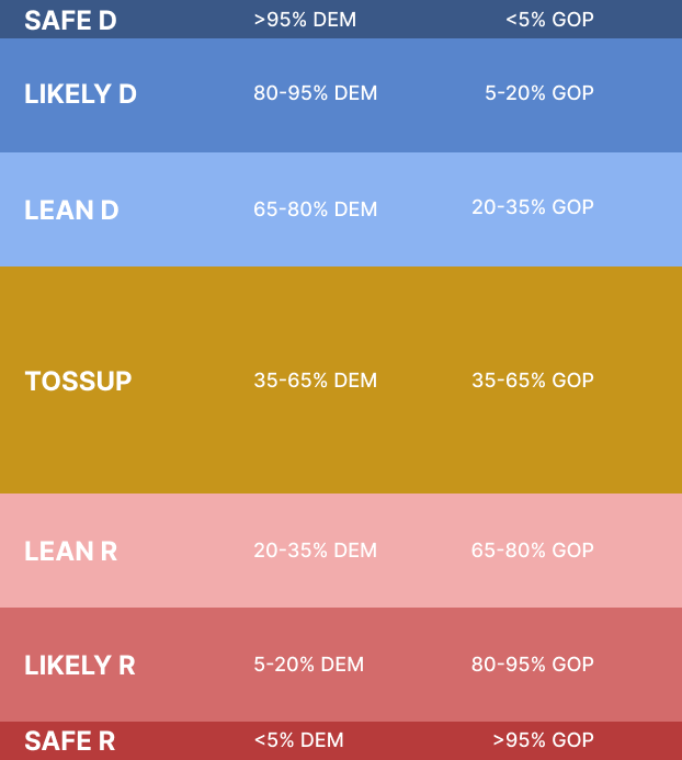
Figure 1
Blended Poll Averages
In our forecasting model, we employ a blended averaging method that includes data from every presidential horse race and head-to-head poll that comes out by a pollster with different polling dates. This blended average approach calculates the national and state-level averages of candidate support using a cubic spline. This ensures that we include every unique poll conducted into the overall average, while minimizing the influence of biased or outlier polls, and polling frequency disparities.
Poll Weighting
DDHQ has adjusted our election forecasting model by introducing a dynamic approach to weighting state polls and fundamental indicators as the election date approaches. The overall structure of the model remains consistent, with only the future trajectory of the weighting balance being modified. With this launch, the model reduces poll related uncertainty over time by applying an exponential decay factor to fundamental indicators, such that polls have more weight in the predictions the closer to Election Day we are. Moreover, the model factors in the number of polls a specific race has and poll weights are gradually increased as more polls become available. This approach improves weighting without introducing any discontinuities and better reflects the increasing relevance of polling data as the election nears.
Dataset and Variables
Our Congressional model draws from a large base dataset of 265 variables in the House and 201 in the Senate, spanning each non-special congressional election from 2006 through 2020. A list of these variables and their sources can be found here .
In addition to primary source data, we also feature-engineer several important variables. Our national environment relies on using a weighted average of generic ballot polling, built to account for pollster bias and variability. In addition to regular FEC numbers from campaign reports, we also incorporate a formula to compare Republican and Democratic campaign finance numbers in each district/state. As Michael Bloomberg and Tom Steyer know very well, increasing funding comes with diminishing returns for every extra dollar. We account for this by taking the difference in logarithms of the Democratic and Republican candidates' fundraising. Polling data for each race is consolidated using a weighted average that accounts for recency, pollster bias and pollster quality. Our polling average does not change unless new polls are added, so in the early stages of a race, our polling average may appear static.
We refresh the dataset on a rolling basis to ensure that any and all changes to individual races are accounted for quickly. This includes adding any new individual race polling, changes in the national environment and special election environment variables, quarterly and 48-hour FEC reports, new economic indicators, primary election outcomes, and candidate status changes. For our weekly public update, the dataset will encompass all changes available at the end of the previous Friday, plus any polls released by the day before the update.
Prediction Framework
We assembled data from previous elections dating back to 2006 as our training set for our Senate and House models. However, on the Senate side, there have only been a few hundred Senate races to train a model on - not very many when one considers that even in our condensed model we are using dozens of variables. To rectify this, we also use previous House elections to help train our Senate as well as our House models. This leads to a much more stable and confident fit for our models, and also allows us to make distinctions between elections in the two chambers of Congress.
More recent elections are weighted more heavily than older ones to account for evolving political trends that have altered electoral dynamics in recent decades. The Congressional model also emphasizes data from past Presidential election years compared to midterms, as Congressional races in Presidential years show distinct patterns. The model recognizes that cross-party voting has become increasingly rare, particularly in Presidential elections, making it more challenging for candidates to significantly outperform their party's baseline expectations.
Feature Selection
We employ feature selection methods to optimize our ensemble approach, following best practices in computational modeling and academic literature.
Elastic Net: Elastic Net is a blend of LASSO and Ridge regression used for regularization and variable selection. LASSO is useful for high-dimensional datasets because it is computationally fast. However, if there is a group of variables that have high pairwise correlations, then LASSO often selects only one variable from that group, which may lead to “over-regularization”. Elastic Net addresses the problem of “over-regularization” by incorporating a ridge penalty which shrinks the coefficients instead of zeroing them out (Zou and Hastie 2003). Because the predictors have such high pairwise correlations (think 2020 House vs. 2020 Presidential results in the district), we decided to weight the L1 and L2 regularizations equally in our ElasticNet component. This leads to a robust and parsimonious model that provides an excellent component for the eventual Ensemble Model.
Manual Feature Selection: Taking a more subjective approach to feature selection, we can select substantively important variables rather than allowing an algorithm to choose. Quantitative models sometimes fail to capture important differences that are not easily quantifiable or need more subjective adjustments made possible by researchers' discerning eyes. Models predicting Congressional results span the latter half of the 20th century (Stokes and Miller 1962; Tufte 1975; Lewis-Beck and Rice 1984) with relatively simple quantitative analyses and are still relevant and accurate through the work of contemporary scholars (Campbell 2010; Lewis-Beck and Tien 2014). We choose to include many of the same variables that these researchers find most important, such as incumbency (Erikson 1971; Abramowitz 1975), district partisanship (Brady et al. 2000; Theriault 1998), and whether a given year is a midterm or Presidential cycle (Erikson 1988; Lewis-Beck and Tien 2014). At the same time, adhering to the Principle of Parsimony, we exclude relatively minor variables for which we do not have a strong theoretical reason to believe they substantially affect most election results, such as average wages. Also, while scholars typically fail to find a general causal linkage between raising more money and winning, it does appear to be a considerably predictive variable for challenger success (Jacobson 1978).
Algorithms
Most election forecasting models utilize either a Bayesian approach or classical logistic regression to predict the outcome of an election. Our modeling process has evolved to utilize an ensemble technique, incorporating various algorithms and variable subsets, including Bayesian ridge regression, linear regression, Random Forest, XGBoost and Elastic Net to forecast an election. Including a variety of algorithms and variable subsets in our ensemble reduces error in two ways. First, ensembles have proven to be more accurate on average than their constituent models alone. Second, they are less prone to making substantial errors (if they miss, they miss by smaller margins on average) (Montgomery et al. 2011). Individual models produce good results, but will give slightly different estimates for each race. On the whole, we have found them to be comparable based on various accuracy metrics, but they produce better estimates when averaged together. In our testing, the ensemble predictions produce fewer misses in 2014 and 2016 than any single model alone.
In the House model, we combine two separate ensemble models to leverage both party-oriented variables as well as incumbency-based variables, and then add any recent polling information. In the Senate, a single party-oriented ensemble model is sufficient to produce accurate results, and is later combined with polls to make a final prediction.
Each algorithm is listed and briefly described below.
Bayesian statistics, in a simplified manner, consists of utilizing observed data to update our degree of belief in an event occurring. For our purposes, the outcome of a particular race is modeled as a normal random variable with margin θ. The margin θ is modeled as a function of the features in the dataset using linear regression. Parameters of the linear regression are drawn from non-informative prior distributions, such as the Cauchy distribution, a distribution with extremely heavy tails, and which has a higher chance of sampling unlikely events.
Random Forest is a well-known tree-based algorithm. It produces an estimate for each race by walking through many decision trees and then outputting the mean predicted margin of these trees.
XGBoost is an ensemble trees algorithm that uses the gradient boosting library. As with Random Forest, it can be utilized for supervised learning tasks such as our forecasting model.
Linear Regression finds the optimal (least-squares) combination of factors which best predicts the eventual margin in a race. We use a weighting scheme that gives more weight to close elections, so our model can train the most on the key races.
Elastic Net is a mixture of LASSO and ridge regression. LASSO regression (L1 regularization) applies a penalty to reduce the number of variables, and ridge regression (L2 regularization) applies a bias term that reduces the volatility of the predictors and is most useful when the predictors are highly correlated with each other (as is true in our case).
Polling and the Decision Desk HQ Poll Average
Decision Desk HQ internally collects polls and creates a polling average used in the forecasting model. The approach incorporates all available public and internal polls into the Decision Desk HQ polling database. An adjusted cubic spline interpolation technique creates a smooth and continuous curve between data points, minimizing abrupt changes in any direction. The methodology involves daily fitting of new cubic splines, incorporating historical and new data points while preserving the integrity of past averages. Without any new polls in a day, the polling average remains constant, reflecting the most recent available data. This methodology enables Decision Desk HQ to deliver reliable and comprehensive polling averages that accurately reflect the sentiment of the electorate across various political races and indicators.
The final forecast predictions are derived from a weighted average of two components: the fundamentals, which include all relevant data inputs except polls, and the polling average. The model determines the optimal weightings for these factors based on historical training data.
Dynamic Modeling
Race-level forecasts also consider the time remaining until the Presidential election. As the election approaches, the model dynamically adjusts its weightings to emphasize polling data, as polls become increasingly predictive of the outcome. Conversely, when the election is further away, the forecast relies more heavily on fundamental metrics, acknowledging that polling data is more likely to fluctuate and that sudden changes in dynamics can occur. The model's probabilities also become more certain closer to Election Day, reflecting the increased stability of race-level and generic ballot polling as the event draws near.
Election Simulations
After calculating probabilities for each individual Presidential state, House and Senate race, we then turn our attention to predicting the aggregate number of electoral votes/seats we expect the GOP to win and the probability of winning the Electoral College and taking control of the House and Senate. We use each race's predicted probability and margin to run simulations of the 2024 elections.
Presidential race results by state are not independent from one another. For example, the candidates are the same, and polling errors are likely to be correlated. By treating each state as an independent entity, such suboptimal models neglect the potential for systematic polling errors or shifts in the national political environment that could similarly affect multiple states. This oversight led to a notable instance where one forecast designer found himself in the unenviable position of having to consume a bug on live TV, as a consequence of his model's overconfident prediction that Hillary Clinton would defeat Donald Trump in 2016. To account for the relationships across states and the importance of these correlations, the DDHQ modeling team implements a realistic and robust correlated simulation process.
Similarly, many election forecasters erroneously consider the outcome of each Congressional race to be independent of others; however, in reality, this is NOT the case. Polling errors and national environment errors are mildly correlated across Congressional races within an election cycle due to various sources of error, resulting in systematic bias (Shirani-Mehr et al. 2018).
In the Presidential simulation, we employ a multi-level approach incorporating national, regional, and race-level stochastic noise to create a realistic pairwise correlation structure in our model. In the Congressional simulation, we include national and race-level stochastic noise.
At the national level, we generate a random variable representing the overall political climate, which affects all races simultaneously. This variable is drawn from a normal distribution with a mean of zero and a carefully chosen standard deviation that reflects the historical variability of national polling errors. Next, we divide the country into distinct regions based on geographic and political similarities. We employed hierarchical clustering techniques to determine the optimal regional groupings for our multi-level simulation approach. By analyzing a comprehensive set of demographic, geographic, and political variables that could potentially influence the correlation of polling and other forecast errors, we divided the United States into 10 distinct regions. We generate a regional random effect for each region in each simulation, also drawn from a normal distribution with a mean of zero and a region-specific standard deviation. These regional effects capture the shared characteristics and correlations among races within the same region. Finally, we incorporate race-specific random noise for each individual contest, accounting for the unique factors and race-level polling errors that may affect each race differently.
Combining these three levels of random effects - national, regional, and race-specific - we create a robust and realistic simulation process that accurately captures the complex correlations between races (see Figure 2). We run millions of daily simulations to calculate the probabilities of Democrats or Republicans winning the Presidency, Senate and House and the likelihood of each possible combination of outcomes across these three chambers (see Figure 3).
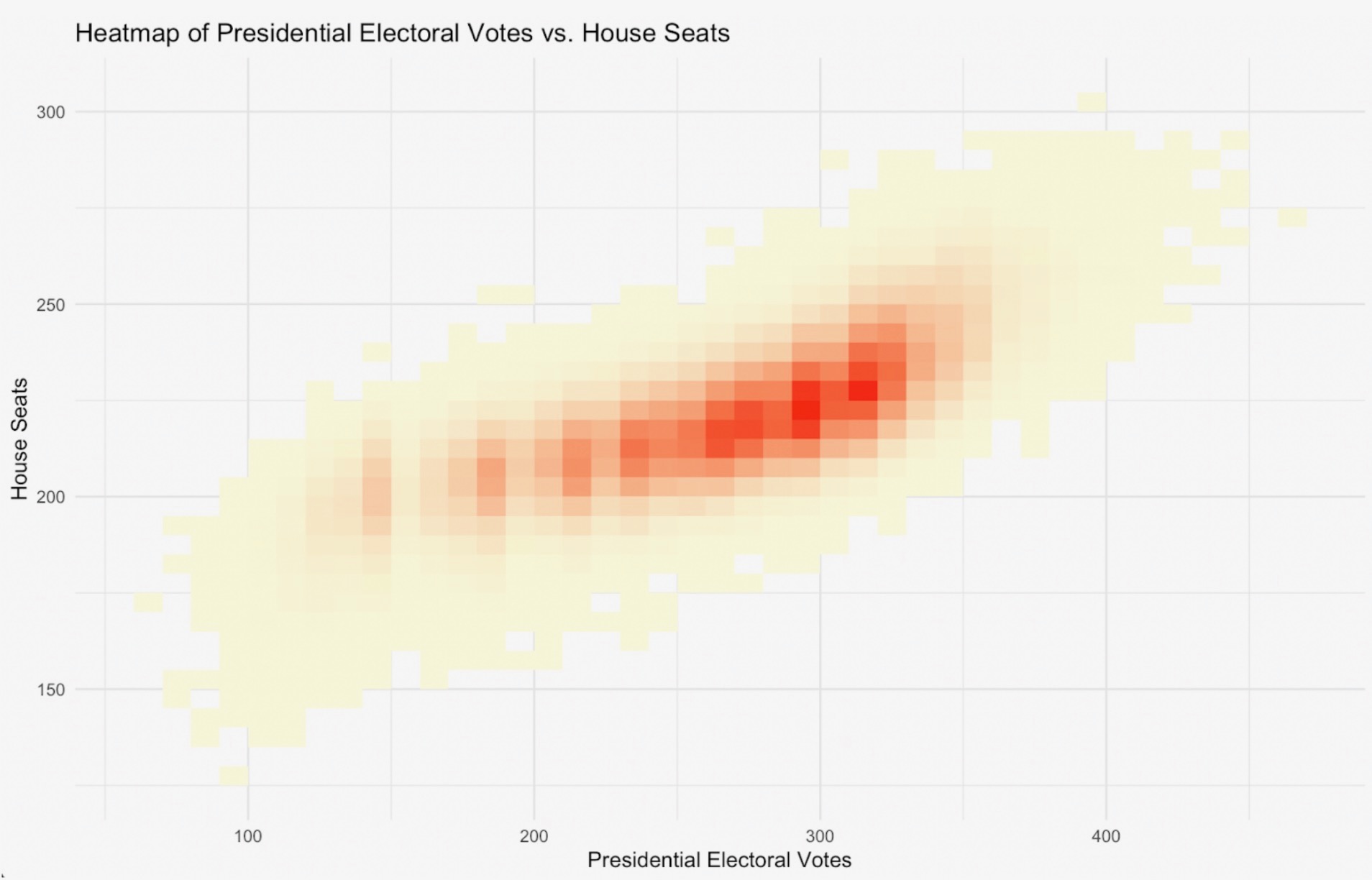
Figure 2
Figure 3